Key idea:
The climate model you just ran moves carbon between three reservoirs on your planet:
the atmosphere, the ocean and the solid sediment. This is the carbon cycle described above.
Carbon moves between these three reservoirs at
rates that depend on your chosen parameters. The weathering rate (that moves carbon from the atmosphere
to the ocean) depends on the land fraction and average surface temperature. Meanwhile, volcanism & degassing
returns carbon from the sediment to the atmosphere and is affected by your choice for your planet's volcanism.
The sedimentation rate moves carbon from the ocean to the sediment, and changes depending on the fraction of carbon stored
in the ocean (altered by weathering).
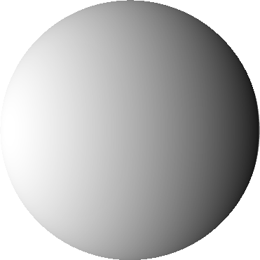
The picture above shows a diagram of this model. The arrow size and colour for weathering and volcanism & degassing
change depending on your parameter choices. Fatter arrows represent a larger initial flux of carbon between reservoirs, while blue and red indicates
a cooling or warming effect compared to present-day Earth (the sedimentation flow is initially always the same as present-day Earth, but will change
in proportion to the abundance of carbon in the ocean increasing or decreasing). Put your planet closer to the inner habitable zone edge or give the planet more land,
and the weathering rate will increase to cool the planet. Bump up the volcanism and the planet will start to warm as carbon is pumped
into the atmosphere. Eventually, these fluxes will balance and your planet will reach its new average surface temperature.
The average surface temperature is calculated from the amount of carbon in the atmosphere (which forms the greenhouse gas,
carbon dioxide) and the radiation from the star (determined your choice of position within the habitable zone). The surface temperature
also assumes additional heating from water vapour, which is another greenhouse gas.
Shuffling carbon:
Your planet initially begins as a present day Earth, with the carbon reservoirs and surface temperature taken from global estimates.
Your choices for your new planet properties changes the weathering and volcanism rates and carbon starts to move between the reservoirs.
This alters the amount of carbon in the atmosphere and the surface temperature changes. Eventually, the carbon cycle reaches a new balance
point where the amount of carbon entering and leaving each reservoir becomes constant. We call this point equilibrium. The surface
temperature at equilibrium is the new global temperature of your Earth-like world.
You can see your planet evolve to its new state on the plot to the right. The ocean and sediment reservoirs contain the greatest quantities
of carbon, so they change relatively little compared to the atmosphere.
Depending on how different your planet is from the Earth today, it may take a long or short time to reach equilibrium. If the graph never
flattens to a constant value, then equilibrium has not been achieved within the time limit for this model. The surface temperature is then a
lower or upper limit (depending on if the graph is rising or falling).
You can download the data of your planet's evolution by pressing the "Download data" button underneath the graph. This is
handy if you want to compare models by plotting them yourself. Due to disc space, the data is available for 5 minutes after the page
is loaded. Need it again? Just reload the page.
Of note:
This model must always have three carbon reservoirs, so it is not actually possible to consider a completely dry planet or an ocean world with no
exposed land. In the case where land fraction is 1.0, it can be assumed there is water beneath the surface providing the reservoir. For a near-ocean world
(very tiny land fraction), weathering is throttled so the code may never reach equilibrium. The temperature recorded is therefore a lower limit and the
planet will actually get hotter. In reality, secondary mechanisms could kick-in on ocean worlds, such as evaporation exposing land once again. You might also be
interested in checking out our F.A.Q. for other fun facts about this model.
Show me the maths!
If this description was insufficient to quench your curiosity, we can describe the model quantitively.
The carbon in each reservoir (R) is found by integrating the following four equations over time:
\[{dR_{\rm atm} \over dt} = F_{\rm vol} - F_{\rm w} \]
\[{dR_{\rm oce} \over dt} = F_{\rm w} - F_{\rm sed} \]
\[{dR_{\rm sed} \over dt} = F_{\rm sed} - F_{\rm vol} \]
\[{dR_{\rm atm} \over dt} + {dR_{\rm oce} \over dt} + {dR_{\rm sed} \over dt}= 0\]
The first three equations describe how carbon changes in each reservoir over time. The atmosphere reservoir
(\(R_{\rm atm} \)) gains carbon due to the flux from volcanism & degassing (\( F_{\rm vol} \)) and loses it through
the flux due to weathering (\( F_{\rm w} \)). Similarly, the ocean reservoir (\(R_{\rm oce} \)) gains carbon from weathering but
loses it through sedimentation (\( F_{\rm sed} \)). Finally, the sediment reservoir gains carbon from sedimentation and loses it through
volcanism & degassing (\( F_{\rm vol} \)). The final equation says all of these changes need to add to zero, as no carbon is lost or gained from the planet.
Weathering is the most complex of the fluxes, as it depends on the land fraction, \(\gamma\), the abundance of carbon in the atmosphere reservoir, \(R_{\rm atm}\), and the
surface temperature, \(T_s\). The form is the same as in previously published works such as Abbot et al. (2012):
\[F_{\rm w} = F_{\rm w, \oplus}\left(\frac{\gamma}{\gamma_\oplus}\right)\left(\frac{R_{\rm atm}}{R_{\rm atm,\oplus}}\right)^\beta e^{(T_s - T_{s,\oplus})/k}\]
The parameters with a \(\oplus\) subscript denote a constant equal to that value on present-day Earth (the starting point for the new world). The index \(\beta = 0.165\) is a rate constant that
controls how sensitive the weathering is to the abundance of carbon in the atmosphere. Similarly, \(k = 10\)K (\(-254.15^\circ\)C) and controls how sensitive the weathering is to
the surface temperature.
The surface temperature is calculated from the abundance of carbon in the atmosphere via a parameterisation developed by Walker et al. (1981):
\[T_s = T_{s, \oplus} + 2(T_{\rm eq} - T_{\rm eq, \oplus}) + 4.6\left(\frac{R_{\rm atm}}{R_{\rm atm, \oplus}}\right)^{0.364} - 4.6 \]
\(T_{\rm eq}\) is the temperature of the planet at the top of the atmosphere, i.e. the temperature purely based on the radiation from the star without the effect of the greenhouse gases in
the atmosphere. For the Earth, our \(T_{\rm eq}\) is a very chilly \(-18^\circ\)C, but our atmosphere traps heat to give a global surface average of about \(15^\circ\)C. The equilibrium temperature is given by:
\[T_{\rm eq} = (1 - \alpha)\left(\frac{L_\odot}{16\pi\sigma a^2}\right)^{1/4}\]
Here, \(\alpha\) is the albedo or reflectivity of the planet, which determines how much radiation is reflected back into space. For the Earth \(\alpha = 0.3\). This value rises as the average surface
temperature drops below 273.15K (\(0^\circ\)C) and the planet begins to become covered with ice. Below 250K (\(-23^\circ\)C), the albedo reaches 0.6, a value consistent with an icy world such as the Jovian moon, Europa.
The fluxes for sedimentation and volcanism & outgassing are more simply proportional to the abundance of carbon in the oceans and sediment, multiplied by the rate at which carbon
is leaving the atmosphere on present-day Earth (weathering, \(F_{\rm w, \oplus}\)):
\[F_{\rm sed} = F_{\rm w, \oplus}\frac{R_{\rm oce}}{R_{\rm oce, \oplus}}\]
\[F_{\rm vol} = \Gamma F_{\rm w, \oplus}\frac{R_{\rm sed}}{R_{\rm sed, \oplus}}\]
The rate of volcanism & degassing can be increased or slowed by the factor \(\Gamma\) that is your chosen volcanism in the model.
A examination of the model performance and how the surface temperature varies with difference choices for the planet conditions can be found
in the Earth-like paper, published in the International Journal of Astrobiology (Tasker et al. IJA 2020: preprint here). Our F.A.Q. is also worth a look.